Preface
A while back I was peer-reviewing a trading strategies research paper, I became bottle-necked by an AdaBoost Decision Tree Stump Analysis that was clocking over ~10 minutes to complete. As this part of my analysis was only one-third of the analyses that I was conducting, for logistical, spiritual reasons – I had to remedy this bottleneck. An immediate solution was utilizing the parallel processing packages: foreach(), and doMC().
foreach and doMC Packages
The foreach package supports parallel execution. The foreach function is just a for loop, but it returns objects e.g. lists(), matrices, and arrays. A reason for using foreach package over other looping functions i.e. the apply family is that foreach supports parallel execution. The doMC package provides the mechanism for the foreach function. The doMC package only works on a single computer, NOT a cluster of computers. I found this out the hard way.
To run a parallel job, you simply add %dopar% after initializing the cluster object.
registerDoMC(2)                                               #initialize cluster object
foreach(i=1:4, .combine='+') %do%    {some_function(i)}       #sequential
foreach(i=1:4, .combine='+') %dopar% {some_function(i)}       #parallel
Seems simple, no? But there are a lot of potential pitfalls. foreach function works best when different tasks can be done independently, but when these tasks have to communicate with each other, then foreach function can be quite inefficient. I too found this out the hard way.
A Simple Example
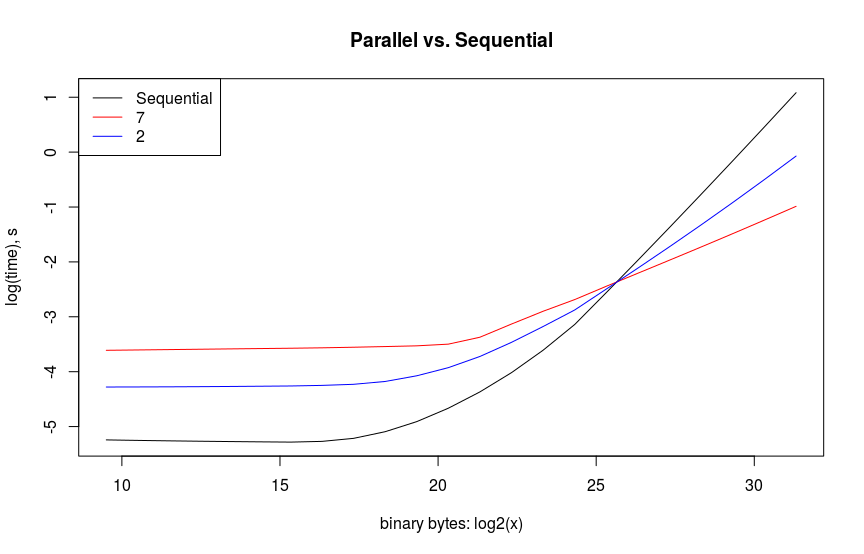
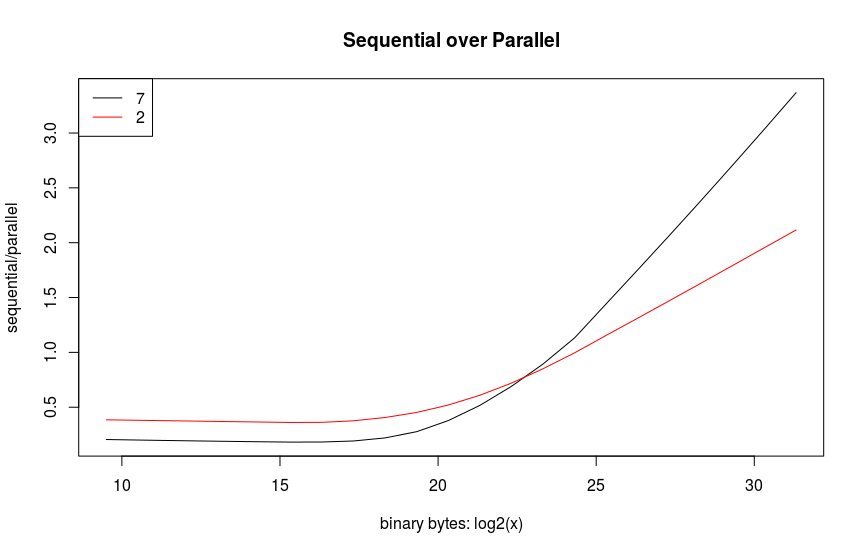
The example that I chose to show here is simply calculating the Frobenius norm of a varying sized list of vectors. Believe it or not, trying to recreate this example to run as my model had done was actually more educational than the original application. I chose this example because it is similar to baseline matrix multiplications which are typically used for comparing performance. My computer only has 2 cores, so to get something more exciting and expensive, I used an EC2 instance. Amazon charged me $\$0.44$ to run this. I guess I could’ve bought a Bazooka Joe instead – if those still exist. The results below show the expected overhead in parallelizing small vectors. Spinning up more task takes up more time for smaller sized objects. This seems evident when comparing the red, blue, and black lines below. Likewise, a performance gain for parallelizing is only observed after the object’s size is over $2^{25}$. The parallelization doesn’t quite meet the available number of cores, but this most likely due to inefficient code on my part with a nested loop thereby reducing the number of cores that are available. This will be a follow-on exercise for me to verify.